

How FiniteNow Works: Getting Quotes for your Simulation in Minutes
Getting your simulation project started is straightforward. Our guided workflow captures the essential technical details step by step – from defining your project scope to receiving a transparent proposal. Each section focuses on the information that matters most for accurate and efficient analysis, so you can move from concept to results without unnecessary overhead.
Summary: What is a Fatigue Analysis?
Fatigue occurs when the strength of a product decreases over time as it undergoes repeated loads; this differs from monotonic fracture behavior observed during an initial load.
The State-of-the-Art Modeling Approaches
The current method of fatigue analysis separates the product’s fatigue life into the number of cycles the product has endured before failing, into two main types: high-cycle fatigue (typically involving only elastic deformation in tensile stress up to 10 8 cycles) and low-cycle fatigue (involving plastic deformation in tensile stress for less than 10 4 cycles). High-cycle fatigue is typically analyzed using the stress-life (S-N) method, whereas low-cycle fatigue is analyzed using the strain-life (ε-N) method.
In all cases, fatigue failure proceeds by the formation of cracks within the component (usually initiated by a localized stress concentration or a microstructural defect) and subsequent cracking. Though both the S-N and eplison-N method inform about the accumulated damage over given loadcycles, they do not resolve the physical crack formation. Linear-Elastic Fracture Mechanics (LEFM) and Elastic-Plastic Fracture Mechanics (EPFM) need be used to analyze localized cracking once it has formed.
Additionally, all forms of multiaxial stresses, mean stresses, and any type of notch significantly impact a product’s lifespan and therefore need to be accounted for through a variety of means such as critical plane methods (i.e. Fatemi-Socie), and empirical correction methods (such as Goodman, Smith-Watson-Topper).
An important precessing step is the aggregation of a complex loadin behavior into a representative load cycle. Here, rainflow counting can be used to convert sequences of variable-stress loads into an equivalent number of constant-amplitude cycles. Then, Miner’s Rule is employed to accumulate the damage over multiple different such load cycles.
Why FEA enables Fatigue Prediction
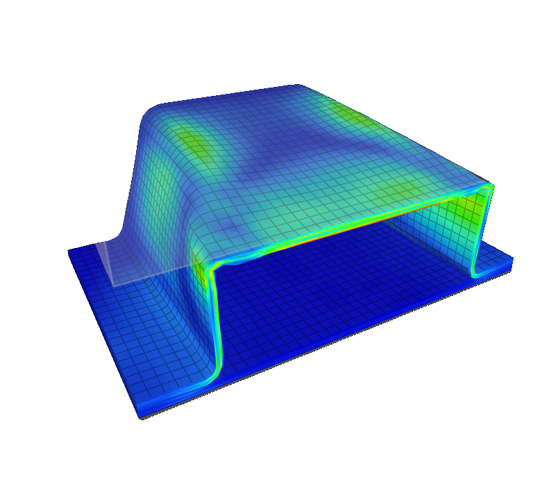
Finite Element Analysis (FEA) is the foundational tool to predict fatigue life. For HCF, linear FEA allows engineers to determine the local cyclic stress-strain fields of their designs and thus determine the global or “hot-spot” stresses at various points throughout a design. These values are then inputted into established S-N curves to establish the potential fatigue life of a particular part. Likewise, for strain-based approaches nonlinear FEA strains and known material cyclic properties are used to predict the fatigue life of a design under LCF. Cracking can also be predicted using FEA techniques (e.g. Virtual Crack Closure Technique (VCCT), cohesive-zone models, or XFEM) through the Paris–Erdogan equation.
How the different Industries treat Durability
Industrial practice varies by sector: aerospace typically enforces damage-tolerance analysis with prescribed load spectra (e.g. FAA AC 23-13A fuelair-ground cycles) , automotive uses FEA-based S–N/durability methods aligned with component testing, and energy/pressure-vessel industries rely on code fatigue curves (ASME, DNV) augmented by FEA refinement . While modern FEA tools and advanced methods (e.g. two-stage total-life models, multiscale simulation) continue to improve accuracy, fatigue life predictions remain uncertain due to material scatter and modelling assumptions, so design codes employ conservative factors .
Why FiniteNow is your Fatigue Expert
With advanced finite element analysis (FEA) services, engineers can design safer, lighter, and longer-lasting products while reducing the cost and time of physical testing.
At FiniteNow.com, durability and fatigue analysis is performed using industry-grade FEA workflows tailored for metals, composites, and hybrid materials. We supply stress-life, strain-life, crack-growth, and custom solutions. By combining instant project quoting, scalable engineering teams, and cost-efficient delivery from pre-audited simulation providers, FiniteNow ensures fatigue simulations are accessible, fast, and reliable.
Durability Simulation: Thinking longterm.
The main goal of fatigue analysis in structural simulation is to estimate how long a part will last under real-world cyclic loads. While static FEA can confirm a design does not fail under peak stresses, durability simulation goes further by calculating crack initiation, crack growth rates, and lifetime under variable load spectra.
Typical targets include:
- Predicting fatigue life under constant amplitude or random loading.
- Identifying weak spots and stress concentrators where cracks are most likely to form.
- Improving durability by design optimization, such as geometry adjustments or surface treatments.
- Supporting certification requirements, e.g., in aerospace and automotive, where fatigue validation is mandatory.
For engineers, durability simulation is not only about preventing failures, but also about enabling weight reduction and cost efficiency by using materials to their maximum potential without compromising safety.
How we approach Fatigue and Durability
Linear elastic FEA is often sufficient to calculate stresses for early fatigue screening. However, for components with local plasticity, nonlinear analysis is required to capture strain ranges accurately. Nonlinear finite element analysis provides better estimates for low-cycle fatigue, where materials yield repeatedly. Experienced analysts often combine both approaches, using linear FEA for global screening and nonlinear simulations for critical hot spots.
Durability analysis can be conducted in the time domain using actual load histories, such as road load data or service load spectra. Time-based fatigue analysis accounts for variable loading and sequence effects, which are critical in automotive or wind turbine components. Frequency domain methods, on the other hand, allow faster evaluation under random vibration loading. Engineers often switch between time and frequency domain FEA depending on the application and test data availability.
Most fatigue analyses rely on implicit solvers, as the stress history is evaluated under quasi-static conditions. However, explicit solvers become necessary when components are subjected to impact, crash, or transient loads, which may accelerate fatigue damage accumulation. For expert users, combining implicit and explicit analyses in a single workflow allows both global durability checks and local transient effects to be captured.
Material modeling is critical in fatigue simulation. Metals are often evaluated with S–N curves (stress-life), while strain-life (ε–N) methods are applied when plasticity dominates. Composites require progressive damage models, accounting for matrix cracking and fiber breakage. Experts integrate environmental effects, such as temperature and corrosion, into fatigue material data, ensuring simulations capture real service conditions.
Stress concentrations at notches, welds, or fillets are the most common fatigue initiation sites. High mesh resolution in these regions is essential to capture local stress gradients. Advanced workflows may combine global–local modeling: coarse FEA models for overall load distribution, refined submodels for fatigue hot spots. Mesh refinement studies are crucial to ensure convergence of fatigue results.
Fatigue often interacts with thermal, fluid, or vibration phenomena. Thermal fatigue occurs in engines and electronics due to repeated heating and cooling cycles. Corrosion fatigue involves chemical degradation combined with cyclic stress. Fluid–structure interaction simulations may be required to model fatigue in turbines, propellers, or biomedical implants. Advanced multiphysics FEA provides realistic predictions for these complex cases.
Deterministic fatigue analysis provides a single life estimate for a given load spectrum. However, variability in material properties, manufacturing defects, and load histories means probabilistic fatigue analysis is often more realistic. By simulating many scenarios, engineers obtain life distributions and reliability curves. These insights support risk-based design decisions and safety certifications.
1D beam models may be sufficient for early durability checks, but 2D and 3D FEA models are required for complex geometries with multiple stress raisers. Shell elements capture weld seams efficiently, while 3D solid elements are necessary for local crack initiation studies. Advanced fatigue workflows integrate crack propagation simulations using XFEM or cohesive elements.
Frequency domain fatigue analysis is efficient for vibration-driven fatigue, such as in aerospace structures or electronic assemblies. Time domain analysis is better suited for variable amplitude road loads, wind spectra, or operational histories. Engineers often calibrate frequency domain fatigue predictions against time-domain simulations to validate their accuracy.
Modern fatigue analysis is increasingly automated. Engineers can link durability simulations with design optimization algorithms to minimize weight while maintaining target life. Automated workflows can scan multiple load spectra, materials, and geometries to identify the most durable configurations. This reduces manual iterations and speeds up decision-making in product development.
Solver strategies depend on whether the goal is life prediction or crack propagation. Stress–life and strain–life fatigue use implicit static solvers, while fracture mechanics–based fatigue may require nonlinear transient solvers. Hybrid workflows combine both approaches, ensuring accurate predictions across different fatigue regimes.
Most fatigue FEA assumes continuum damage accumulation until a predefined crack initiation point. Discrete crack modeling, such as XFEM or cohesive elements, explicitly simulates crack initiation and growth. Advanced workflows integrate both methods: continuum FEA for crack initiation, followed by discrete crack growth modeling to estimate residual life.
How FiniteNow avoids typical Mistakes in Fatigue Simulations
One common mistake is relying solely on static stress results to estimate fatigue life, without considering load spectra or material strain ranges. Another is neglecting mesh refinement at notches or welds, leading to overly optimistic fatigue predictions. Many engineers also overlook environmental influences such as corrosion, which can drastically reduce durability.
To avoid these pitfalls, engineers should always calibrate simulations with experimental fatigue data, apply appropriate material models, and validate results with physical testing when possible. Automated workflows and sensitivity studies can further reduce uncertainty. Leveraging expert FEA services, like those at FiniteNow.com, ensures best practices are applied consistently across projects.


Use Cases for Fatigue
Automotive – Suspension Component Fatigue
Suspension arms and brackets experience millions of cycles under variable road loads. FEA-based durability analysis ensures they last the vehicle’s lifetime without cracking. By combining road load data with fatigue simulations, manufacturers reduce warranty claims and optimize weight.
Aerospace – Wing and Fuselage Durability
Aircraft wings and fuselage panels are exposed to cyclic pressurization and aerodynamic loads. Fatigue simulation with FEA helps predict crack initiation in riveted joints and composite laminates. This enables predictive maintenance schedules and compliance with strict aviation regulations.
Energy – Wind Turbine Blade Fatigue
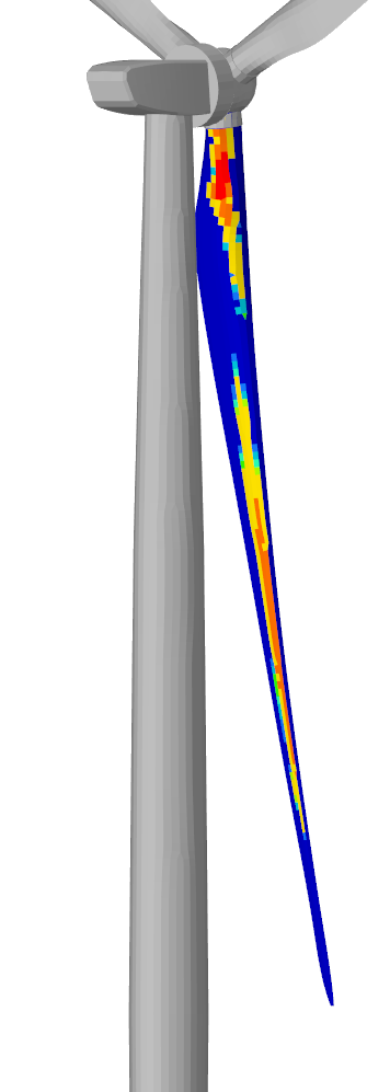
Wind turbine blades are subjected to highly variable wind loads, leading to cyclic stresses in composite materials. Finite element fatigue simulations assess durability under both aerodynamic and gravitational loads. Accurate predictions extend service life and reduce costly downtime.
Learn more about our portfolio of Structural Engineering Services
Stages of Fatigue in Metal Materials
Fatigue is progressive damage in metallic materials under cyclic loading that goes through different physical stages. Fatigue does not occur through monotonic failure; instead, it develops after multiple load cycles and is controlled by the material’s microstructure, the local stress-strain state, and crack-growth properties. The four main stages of fatigue used in most analyses conducted in engineering practice and finite element-based fatigue analysis are listed below:
From Initiation to Failure – A Process Overview
Fatigue starts at the microscale, where cyclic loading produces localized plastic deformation in regions of high stress, even when the nominal stress is below the macroscopic yield strength. Persistent Slip Bands (PSB) form in individual grains from localized cyclic shear deformation. These PSBs create surface intrusions and extrusions that function as stress concentrations. Following multiple cycles, microcracks will develop at these locations, including:
- grain boundary intersections
- inclusions or second-phase particles
- surface defects (i.e., surface scratches) or machining marks
- geometric discontinuities (e.g., notches, weld toes)
High-Cycle Fatigue (HCF) has initiation as the dominant component of total fatigue life, as it may take millions of cycles for crack initiation to occur. Low-Cycle Fatigue (LCF) has initiation occurring rapidly due to large amounts of plastic strain.
N total ≈ N initiation + N propagation
Classical Stress-Life Methods consider both the initiation and early growth stages of fatigue combined as part of empirical S-N Curves.
Once a microcrack forms, it grows under subsequent cyclic loads. At this point, the crack generally spans a few grain sizes. It is during this time that the crack’s behavior is strongly influenced by the material’s microstructure. Characteristics of short cracks include:
- Growth below the long-crack threshold
- Sensitive to microstructural barriers (grain boundaries and/or phase interfaces)
- Nonlinear and accelerating growth rates
This is a transitional stage between crack initiation and traditional fracture-mechanics-based final failure. Linear Elastic Fracture-Mechanics (LEFM) does not adequately describe this regime because the plastic zone around the crack tip is comparable in size to the growing crack.
For modeling purposes, this regime is difficult to model directly in FE and is thus often modeled indirectly through total-fatigue-life methods or, alternatively, through Equivalent Initial Flaw Size (EIFS) concepts.
When the developing crack reaches a critical length (generally larger than a few grain diameters), it grows primarily under the influence of the global stress field rather than microstructural factors. During this stage, Linear-Elastic Fracture Mechanics accurately describes crack growth.
The crack-growth rate is represented by the Paris-Erdogan equation:
da/dN = C · (ΔK) m
where:
- da/dN represents crack-growth-per-cycle
- ∆K represents the stress-intensity-factor-range
- C & m represent material-dependent parameters
FEA plays a major role in determining ∆K values or energy-release-rates using techniques such as:
- Virtual Crack Closure Technique (VCCT)
- Extended Finite Element Method (XFEM)
- Cohesive Zone Models
Continued crack-growth continues until the maximum stress-intensity-reach fracture-toughness:
K max ≥ K IC
At this point, unstable-fast-crack-propagation results in sudden final-fracture.
This final stage is characterized by rapid, unstable crack growth after the remaining cross-section cannot support the applied load. This stage is thus much shorter than the entire fatigue life.
Generally, macroscopically fracture-surfaces have:
- fatigue region with beach marks or striations
- overload-zone with either ductile or brittle features
The Engineering Perspective
In practical fatigue analysis with FEA, these stages are generally categorized into two types of analysis methodologies:
| Fatigue Modeling Approach | Crack Initiation | Short Crack Growth | Long Crack Propagation | Material Data Requirement | FEA Integration | Typical Use Case |
|---|---|---|---|---|---|---|
| Stress-Life (S–N) | ✓✓✓ | (✓) | ✗ | ✓ | ✓✓ | High-cycle fatigue, welded structures |
| Strain-Life (ε–N) | ✓✓✓ | ✓✓ | (✓) | ✓✓✓ | ✓✓✓ | Low-cycle fatigue, plasticity-dominated regions |
| Fracture Mechanics (LEFM/EPFM) | ✗ | ✓ | ✓✓✓ | ✓✓ | ✓✓✓ | Damage tolerance, crack growth analysis |
| Total-Life / Two-Stage Models | ✓✓✓ | ✓✓ | ✓✓ | ✓✓✓ | ✓✓✓ | Comprehensive life prediction, aerospace |
| Multiaxial / Critical Plane Methods | ✓✓✓ | ✓✓ | (✓) | ✓✓✓ | ✓✓✓ | Complex loading, non-proportional stress states |
Modern fatigue workflows often employ both methodologies with FEA to compute local stresses and strains for initiation and fracture mechanics for propagation, thus reflecting the multi-staged nature of fatigue failure in metals.
Stress–Life (S–N) and Strain–Life (ε–N) Methods
The S-N and ε–N methods are the most common methods that overview the entire process of fatigue failure; i.e., crack initiation and crack growth. A great method introduction can be found by Schijve.The two methods differ in how they account for material behavior, especially regarding plasticity, but both are closely connected to finite element analysis (FEA) for providing the necessary input data for determining the fatigue lives of structures.
The S-N method is one of the earliest developed fatigue analysis methods. It is best suited for high-cycle fatigue (HCF) where the material’s behavior can be considered purely elastic. A correlation can be established between the stress amplitude and the number of cycles until failure using empirical S-N diagrams.
σ a ↔ N f
Here, the stress amplitude is generally determined from FEA calculations based on a nominal structural (hot-spot), or a local stress range.
The relationship in logarithmic format is generally expressed through Basquins formula:
σ a = σ’ f · (2N f) b
where:
- σ a: Stress Amplitude
- N f : Number of Cycles to Failure
- σ’ f: Fatigue Strength Coefficient
- b : Fatigue Strength Exponent
Practically, FEA is used to calculate cyclic stress ranges at critical locations. Then these stresses are compared with the appropriate S-N diagram of a material or fatigue class (for example, for welded parts). With variable amplitude loads, cycle counting (rainflow) and accumulated damage criteria such as Miner’s rule are applied.
D = Σ (n i / N i)
When D equals 1.0, failure is assumed.
Because of the simplicity of this method and because there are well-established standards for S-N diagrams, it is used very frequently in general-purpose structural engineering, in welding technology, and in all HCF applications. However, it does not explicitly account for local plasticity or notch-root behavior, which limits its applicability in highly stressed or geometrically complex regions.
The ε–N method extends fatigue analysis from the LCF regime to include cyclic plastic deformations. In contrast to the S-N method, this method considers the strain amplitudes instead of stresses.
The strain amplitude is divided into elastically and plastically deformed components. This correlation between strain amplitudes and fatigue life is given by the Coffin-Manson-Basquin equation:
Δε/2 = (σ’ f / E) · (2N f) b + ε’ f · (2N f) c
where:
- E : Youngs Modulus
- ε’ f : Fatigue Ductility Coefficient
- c : Fatigue Ductility Exponent
For FEA workflows, elastic stresses and strains are calculated first. IIf local plasticity is expected (e.g. at notches), corrections such as Neuber’s rule are applied to estimate the true elastic–plastic strain state.
σ el · ε el = σ pl · ε pl
Then the corrected strain amplitude is introduced into the strain-life equation to obtain the fatigue life.
The strain-life method is best suited for:
- Components with high stress concentrations
- Low-cycle or thermomechanical fatigue
- Fatigue cases that involve large amounts of local yielding
The strain-life method is a physically correct representation of the mechanical behavior of materials subjected to cyclic loadings. To use it, however, detailed knowledge of the cyclic stress-strain behavior of a material and its fatigue ductility coefficients is necessary.
Key Differences and Engineering Implications
| Aspect | Stress–Life (S–N) | Strain–Life (ε–N) |
|---|---|---|
| Primary regime | High-cycle fatigue (elastic) | Low-cycle fatigue (plastic) |
| Input parameter | Stress amplitude | Strain amplitude |
| Material behavior | Primarily elastic | Elastic + plastic deformation |
| FEA requirement | Stress field extraction | Strain field + plasticity correction (e.g. Neuber) |
| Notch sensitivity | Limited (empirical correction factors) | Explicitly resolved at local level |
| Material data requirements | Moderate (S–N curves) | High (cyclic stress–strain + fatigue parameters) |
FE Analysis Workflow
Both the S-N and ε–N approaches require FEA. In general, this is done as follows:
- compute the history of stress/strain at the most significant sites,
- apply cycle counting to varying loads,
- calculate fatigue damage using either S-N or e-N relations.
Therefore, the decision to use either the S-N or the e-N model is not mutually exclusive; rather it will depend upon whether there is a localized plastic deformation regime occurring. In numerous cases within industry, engineers have used these models concurrently; that is, they use the S-N model to determine if a part has failed due to high-cycle fatigue throughout its entire volume, then they may choose to examine specific areas where localized plastic deformation occurred during service to further verify their failure mechanism.
Practical Application
From an engineering standpoint, the distinction between the two methods reflects a deeper physical reality. Specifically, fatigue failures occur due to localized cyclic deformations (and subsequent material damage), whereas the magnitude of external stresses acting on the system do not directly relate to the fatigue process. Therefore, while the S-N model can provide an effective, efficient and standardized approach for determining high-cycle fatigue life, it does not account for situations where localized plastic deformations occur. Conversely, the ε–N model provides a more detailed understanding of how localized plastic deformations contribute to fatigue damage, though at increased expendirture in input data (testing) and computation (simulation).
Crack Growth Methods (Fracture Mechanics Approach)
Methods based on fracture mechanics primarily focus on modeling the evolution of cracks under cyclic loading to failure. While they do allow engineers to estimate how long a component can withstand repeated cycles of loading before failing, their primary focus is on describing how a crack grows from an existing flaw (initial crack). As a result, this approach forms the basis for designing “damage-tolerant” structures, i.e., structures designed to tolerate cracks and/or flaws during service (e.g., in aviation applications).
The most significant driving variable is the variation in the stress intensity factor at the crack tip:
ΔK = K max − K min
The Paris-Erdogan equation describes the relationship between fatigue crack growth rate (da/dN), and the variation in the stress intensity factor at the crack tip:
da/dN = C · (ΔK) m
The incremental increase in crack length occurs with each load cycle. The process will continue until the maximum stress intensity factor exceeds the material’s fracture toughness:
K max ≥ K IC
As previously stated, finite element analysis provides a valuable means of estimating crack tip parameters, such as stress intensity factors and energy release rates. Numerical techniques commonly used include:
- Virtual Crack Closure Technique (VCCT)
- Extended Finite Element Method (XFEM)
- Cohesive Zone Models (CZM)
These analyses enable engineers to simulate possible crack path directions and growth rates in response to various real-world loading scenarios.
In general, fatigue crack growth analyses are often performed in conjunction with inspection schedules and some knowledge regarding initial flaw sizes. With this information available, engineers may be able to predict the remaining safe operating time for their components.
Design Concepts for Managing Fatigue Risk
The five main fatigue design concepts provide engineers with a basis for managing the risk of fatigue failure. They represent different ways of thinking about how to deal with the uncertainty associated with fatigue failure; how to address the initiation of cracks in a structural member; and how to manage the risk of crack growth and subsequent failure. Each conceptual framework defines how these uncertainties are addressed during the engineering process. While each represents a distinct way of thinking about fatigue, most engineers today use a combination of these concepts to address their needs — especially in conjunction with finite element analysis. These frameworks provide the overall strategy for applying stress–life (or strain–life) analysis, as well as crack growth analysis.
Safe-life design seeks to guarantee that no cracks form in a component over its lifetime. The safe-life design philosophy aims to ensure that fatigue failure does not occur until a predetermined number of cycles has been reached. Therefore, safe-life designs are typically conservatively sized for cyclic loading to minimize the risk of premature fatigue failure.
N design ≤ N allowable / SF
Key characteristics:
- No cracks are assumed to be present.
- The remaining life of a component is determined using either the S–N or ε–N curves.
- A component is retired from service after its specified lifetime, regardless of whether or not it has deteriorated due to fatigue.
Common applications:
- Rotating machinery.
- Automobile Components.
- Non-redundant structures.
Safe-life is easy to apply, yet it does not account for unexpected flaws or for damage accumulation exceeding initial design assumptions. Consequently, overly conservative designs are often unavoidable.
Damage-tolerant design assumes that cracks develop during the operational lifetime of a component. The focus is therefore placed on ensuring that even if cracks do develop, they will not result in catastrophic failure prior to the next scheduled inspection.
a(t) < a critical for t ≤ inspection interval
Key characteristics:
- Either an initial flaw size is known, or detection occurs.
- Fracture mechanics (i.e., Paris-Erdogan law) is employed to model crack growth.
- Scheduled inspections are performed regularly to detect crack development.
Typical applications:
- Aircraft structural members.
- Pressure vessels.
- Safety-critical Components.
Finite element analysis (FEA) may be employed to calculate stress-intensity factors as well as simulate crack development. A significant increase in safety can be achieved through the application of damage-tolerant design since it allows for explicit management of crack-growth processes. However, the implementation of damage-tolerant design also necessitates a means for performing regular inspections as well as possessing reliable data regarding crack-growth rates.
Fail-safe design incorporates redundant load paths and redistributes loads such that the structural system can endure damage without instantaneous failure.
Key features:
- There are multiple load paths available.
- Failure at a localized point does not immediately cause complete structural failure.
- Often, a fail-safe design includes elements of damage tolerance.
Typical applications:
- Structural members of aircraft fuselages.
- Large civil engineering systems.
Rather than preventing cracks from forming, a fail-safe design is based on a philosophy where failures are gradual and observable, thereby permitting sufficient time for intervention.
With infinite-life designs, components are designed so that operating stresses remain below the fatigue limit. Ideally, this would prevent fatigue failure altogether.
σ a < σ endurance
Key features:
- Only suitable for those metals exhibiting a clearly defined endurance limit (i.e., steel).
- Conservative stress limits are used.
Typical applications:
- Springs, shafts
- long-life mechanical components.
Although this approach is robust, it is not universally applicable, particularly for non-fatigue-limiting alloys such as aluminum.
Because fatigue lives are highly variable, probabilistic design approaches treat fatigue life as a random variable rather than as a fixed quantity.
Key features:
- Accounts for both variability in material properties and loads as well as variability in manufacturing.
- Reliability targets (probability of failure) are established.
- Monte Carlo simulation or other reliability methods are commonly used to implement probabilistic design approaches.
Typical applications:
- High value, high risk systems.
- Design environments driven by optimization.
Probabilistic design acknowledges that there is always some degree of uncertainty associated with fatigue performance and thus facilitates more rational decisions regarding the amount of risk acceptable.
Fatigue of Non-Metallic Materials
The fatigue performance of non-metallic materials differs significantly from that of metallic materials due to fundamental differences in their structures, deformation behavior under cyclic loading, and damage development processes. Still, ultimately, cyclic loading leads to continued degradation and eventually failure; the physics driving failure and the models used to simulate this phenomenon can be much more complex and variable than in metals.
General Characteristics
Unlike most metals, non-metallic materials (e.g., polymers, composites, ceramics) typically do not exhibit metal-like dislocation-driven plasticity. The primary mechanisms that drive fatigue damage in these types of materials include:
- Viscoelastic and/or viscoplastic deformation (polymers)
- Micro-cracking and debonding of fibers/matrix (composite)
- Crack nucleation and propagation in a brittle manner (ceramic)
Another major difference is that fatigue damage in most non-metallic materials often has strong time dependence, i.e., creep, temperature, etc., relative to other material properties.
Polymers and Elastomers
Polymers exhibit fatigue behaviors very similar to those observed in viscoelastic/viscoplastic systems; specifically, the amount of energy dissipated per cycle, or, equivalently, the cyclic softening of the polymer material. For polymers, the response to cyclic loading does not exhibit the same stress or strain dependence as metals. Rather, the cyclic behavior of polymers exhibits dependencies on:
- Loading frequency
- Temperature
- Strain rate
Energy-based approaches are commonly employed to characterize fatigue in polymers, in which the energy dissipated per cycle is related to the remaining fatigue life. Energy dissipated per cycle is given by:
ΔW = ∫σ dε
Chain scission and localized microvoid formation are typical causes of crack initiation. Slow crack growth follows. Tearing energy is a common reference for modeling crack growth in elastomers, rather than the traditional use of the stress intensity factor.
Fiber-Reinforced Composites
Degrieck & Van Paepegem provide a great review of composite fatigue. Crucially, multiscale and anisotropy are inherent features of composite materials. Consequently, composite fatigue involves multiple interacting damage mechanisms:
- Matrix cracking
- Fiber breakage
- Debonding between matrix/fibers
- Delamination between layers/piles
Unlike metals, composites also typically degrade stiffness progressively over cycles rather than through a single dominant crack. As a result, composite fatigue lives are often measured as reductions in stiffness or load-carrying capacity, rather than complete fracture.
FEA-based composite fatigue analysis includes:
- Layered or ply level modeling
- Failure criteria (Hashin/Puck/etc.)
- Damage evolution laws
While S-N curves remain in practical use for composites, they are highly dependent upon lay-up orientation, load direction, and environmental conditions.
Ceramics/Brittle Materials
Ceramics exhibit little to no plasticity and fail by brittle crack growth. Ceramic fatigue is primarily governed by subcritical crack growth under either cyclic or static loading. Here, environmental factors such as temperature and vibration play a dominant role and need to be accounted for in life prediction.
da/dt = A · K n
Due to their predominant deployment in temperature-driven applications, many fatigue assessments also focus on the temperature dependence rather than isolating the mechanical stresses.
However, compared to metals, ceramic fatigue research is still quite sparse, motivating high-fidelity models to break down failure to its most principled root causes.
Modeling & Engineering Implications
Fatigue analysis of non-metallic materials differs from that for metals as follows:
- Less standardized
- More reliance on experimental characterization
- Requires models specific to each material
For FEA applications, this results in moving away from classical stress-based methodologies towards:
- Energy-based damage models
- Progressive damage/stiffness degradation methodologies
- Coupling thermal/mechanical simulation
FAQ: Durability and Fatigue Analysis with FEA Services
Fatigue analysis is the process of predicting how many load cycles a component can withstand before failure occurs. Unlike static strength checks, fatigue simulations consider repeated loading that may cause cracks over time. Engineers use FEA to identify weak points and extend component lifetime. For newcomers, it is often the first step toward reliability-driven design.
A part may withstand a single maximum load but fail after thousands of smaller, repeated loads. Durability simulation ensures a design survives its entire service life under realistic operating conditions. This is particularly critical in automotive, aerospace, and energy applications where long-term reliability is essential. Static strength is necessary, but durability is what prevents in-service failures.
Automotive, aerospace, civil engineering, and energy sectors all depend heavily on durability analysis. Each industry has strict lifetime requirements, ranging from millions of road cycles in cars to 20+ years of service life for wind turbines. Finite Element Analysis Services provide a cost-effective way to meet these demands before physical testing begins.
The stress-life (S–N) method is used when stresses are within elastic limits and high-cycle fatigue dominates. The strain-life (ε–N) method is applied when plastic strains are present, as in low-cycle fatigue. Advanced engineers often combine both methods depending on component hot spots, using FEA to provide local stress or strain histories. This flexibility allows more accurate durability predictions across loading regimes.
Welds, sharp corners, and notches act as stress concentrators, dramatically reducing fatigue life. Without proper modeling and mesh refinement, FEA may underpredict damage in these areas. Intermediate engineers often apply hotspot methods, structural stress approaches, or local submodels to capture weld durability. Fatigue FEA services provide specialized techniques for these critical details.
Real-world loading is rarely constant. Engineers use rainflow counting and cycle counting techniques to convert irregular load histories into equivalent cycles. Time-domain fatigue simulations then apply these load histories to the FEA model. This ensures durability predictions reflect real operational conditions instead of idealized assumptions.
Senior analysts combine fatigue initiation analysis with fracture mechanics–based crack growth simulations. Using stress intensity factors (ΔK) and crack propagation laws, FEA predicts residual life after crack initiation. This integration is vital for safety-critical structures like aircraft fuselages, where inspection intervals depend on accurate crack growth prediction.
Thermal–mechanical fatigue, corrosion fatigue, and fluid–structure fatigue require combining mechanical loading with additional physics. These simulations demand advanced solver strategies and validated multiphysics material data. For experts, multiphysics fatigue is often the frontier where traditional fatigue approaches meet cutting-edge research.
Experts increasingly use probabilistic FEA to quantify fatigue life scatter due to material variability and load uncertainties. Monte Carlo or stochastic methods generate statistical lifetime distributions, which regulators often require for aerospace certification. This goes beyond deterministic safety factors, providing more robust safety margins.
FiniteNow.com offers instant quoting, enabling engineers to start durability projects without lengthy procurement delays. Its network of pre-audited providers ensures high-quality results while maintaining cost efficiency. By offering scalable teams of fatigue experts, FiniteNow matches project size and complexity with the right resources. This combination makes it a unique FEA service provider.
FiniteNow.com uses standardized workflows, validated fatigue libraries, and a pool of senior FEA specialists to maintain consistency. Clients benefit from both speed and technical depth, since projects are reviewed by engineers with domain-specific expertise. Unlike freelance-based platforms, FiniteNow ensures quality through vetted partners and internal checks.
Yes, FiniteNow’s network includes experts in structural–thermal fatigue, vibration fatigue, and corrosion fatigue. Projects can seamlessly scale from single-component fatigue checks to full multiphysics durability simulations. This breadth of capability means clients can rely on one service partner for everything from basic stress-life fatigue to advanced fracture mechanics.
FiniteNow will provide you with a detailed fatigue simulation using finite elements and various fatigue methods (stress-life, strain-life, etc.) to reliably assess the fatigue of your industrial parts.
Yes, FiniteNow has a strong background in simulating various realistic loadings, including multi-axial stresses, variable-amplitude loads, and cycle counting using more sophisticated fatigue models.
FiniteNow can perform fracture mechanics-based analyses, including crack growth modeling via FEA techniques such as the extended finite element method (XFEM) and the evaluation of stress intensity factors.
Yes, FiniteNow allows identifying weak spots and design flaws that contribute to reduced fatigue life. Then we help you find ways to modify the geometry and/or select better materials to increase fatigue resistance.
FiniteNow works in the following sectors: automotive, aerospace, medical, energy & structural engineering, providing the most suitable fatigue methodology for each sector’s needs.
It is best to engage FiniteNow during the initial phases of your project to anticipate potential fatigue problems, but it is also possible to use our services for failure analysis and redesign of existing parts.
Start Now! It will only take 12 minutes
It has never been faster, easier and more cost effective to get a quotation for your structural simulation needs:
Looking for more details and background about Fatigue Analysis?
Durability and Fatigue Analysis with FEA
The Textbook Section
Introduction
Durability and fatigue have long been central concerns in structural engineering. While ultimate strength failures are often dramatic and obvious, it is fatigue that quietly governs the service life of most mechanical and aerospace structures. The crack that initiates at a rivet hole, the weld toe that slowly accumulates micro-damage, the rotating shaft that endures millions of cycles before failure – all of these are governed by fatigue mechanisms.
Finite Element Analysis (FEA) has become a powerful tool in this field. Traditional fatigue design relied heavily on empirical data, S-N curves, and conservative safety factors. With modern FE analysis, engineers can go much further: capturing local stress concentrations, simulating nonlinear material behavior, and even predicting crack initiation and propagation under realistic loading.
For organizations offering FEA services, durability and fatigue analysis represent one of the most valuable applications of the technology. It is not just about proving that a structure survives its first load case, but about ensuring that it will withstand millions of cycles in service, under variable environments and real-world usage.
Fundamentals of Fatigue Behavior
Fatigue is not a single phenomenon but a sequence of stages. First comes crack initiation, often at stress raisers such as notches, weld toes, or fastener holes. Then crack growth dominates, with each load cycle extending the crack incrementally. Finally, once the remaining section is too small, final fracture occurs.
In metals, fatigue behavior is typically described by S-N curves (stress vs. number of cycles). For composites, fatigue is more complex, involving matrix cracking, fiber breakage, and delamination. Regardless of the material, local stress and strain are the driving parameters.
FE analysis plays a key role here. By resolving local stresses and strains under cyclic loading, FEA provides the input to fatigue models. What once required conservative approximations can now be quantified with detailed simulation. For example, FEA can identify which rivet in a joint carries the highest load, which weld experiences the most damaging stress range, or which lug radius is most susceptible to crack initiation.
Durability Analysis with FEA
Durability analysis focuses on whether a structure can meet its design life without failure under expected service loads. This requires not only evaluating stress ranges but also considering real-world loading spectra.
In the automotive industry, for example, durability analysis involves simulating entire proving-ground tracks digitally. Suspension arms, brackets, and body-in-white structures are subjected to load histories derived from measured road loads. In aerospace, flight load spectra are applied, often involving thousands of unique maneuver and gust cases.
FEA enables durability evaluation in two complementary ways. At the global level, system-level FE models determine load distribution across components. At the local level, submodels capture detailed stresses in fatigue-critical features. This “global-to-local” approach is essential: without the global model, loads cannot be correctly distributed; without the local model, stress concentrations cannot be resolved.
Modern FE services frequently integrate durability analysis with multi-body dynamics (MBD) simulations. For example, an automotive suspension system may be represented with flexible FE models of control arms connected to an MBD vehicle model. The interaction between road loads, dynamics, and structural stresses can then be evaluated over millions of cycles, providing a realistic picture of durability performance.
Fatigue Analysis Strategies in FEA
There are several well-established approaches to fatigue analysis within FEA, each suited to different levels of fidelity and computational cost.
1. Stress-Life (S-N) Approach
This is the most widely used method, particularly for high-cycle fatigue. Local stress ranges are extracted from FE results and compared against S-N data for the material. Mean stress corrections may be applied (e.g., Goodman or Gerber).
The method is efficient but assumes that damage is governed by stress amplitude, not strain.
2. Strain-Life (ε-N) Approach
When low-cycle fatigue is relevant, such as in components subject to high plastic strains, the strain-life approach is more accurate. FEA must then resolve local plastic strains, and cyclic plasticity material models may be required.
The Coffin-Manson relation is often used. This approach is common in engines, pressure vessels, and thermally loaded structures.
3. Fracture Mechanics Approach
For components where cracks are expected or already exist, fracture mechanics is used. Instead of predicting when cracks will start, this approach predicts how fast they grow. FEA is used to calculate Stress Intensity Factors (SIFs)
or energy release rates, and crack growth laws such as Paris’ law are applied. This is the standard method in aerospace damage tolerance analysis, where cracks are assumed to exist from the outset.
4. Multiaxial and Non-Proportional Fatigue
Real-world loading is rarely uniaxial. Complex structures may experience combined bending, torsion, and shear. Advanced fatigue analysis methods use critical-plane approaches to evaluate fatigue life under multiaxial loading. FE analysis
provides the local stress tensors, which are then processed by fatigue algorithms to predict damage.
Nonlinear Effects and Contact
One of the key strengths of FEA in fatigue analysis is its ability to capture nonlinear effects. Contact conditions, preload relaxation, friction, and material plasticity all influence fatigue performance.
Consider a bolted joint: if modeled linearly, it may appear that each bolt shares load evenly and experiences moderate stress. But with nonlinear contact and preload included, the analysis may reveal that only a subset of bolts actually carry most of the load, and that micro-slip occurs at the faying surfaces. This localized slip is often where fatigue cracks initiate.
Similarly, in welded joints, the nonlinear redistribution of stresses around the weld toe under cyclic loading may determine the effective hot spot stress. Without nonlinear FEA, such redistributions are lost, leading to unconservative fatigue predictions.
Material Modeling for Durability
Accurate fatigue predictions depend on accurate material models. Metals, composites, and elastomers each require different treatment.
For steels and aluminum alloys, S-N or ε-N curves are widely available. However, scatter is large, and environmental effects such as corrosion or temperature must be accounted for. In composites, fatigue modeling is more complex. Matrix cracking, fiber fatigue, and interlaminar delamination interact in non-linear ways. Cohesive zone models and progressive damage models in FEA are increasingly used to capture these mechanisms.
Elastomers, often used in flexible joints and vibration isolators, exhibit hysteresis and rate-dependent fatigue. Viscoelastic and hyperelastic models in FE solvers can reproduce these behaviors, but calibration against experimental data is mandatory.
Applications Across Industries
In aerospace, fatigue analysis with FEA underpins the entire philosophy of damage tolerance. Components such as lugs, riveted joints, and bonded repairs are analyzed not only for static strength but also for crack growth behavior. Certification authorities require that safe life or fail-safe criteria are demonstrated using validated FE models.
In automotive engineering, fatigue and durability analysis drives design of suspension systems, engine mounts, and welded body structures. Virtual proving grounds are now routine, with FE durability analysis saving enormous cost and time compared to physical prototypes.
In heavy machinery and energy, fatigue governs the life of pressure vessels, pipelines, wind turbine towers, and rotating shafts. FEA enables engineers to model complex load histories and environmental conditions, ensuring reliability over decades of service.
Conclusion
Durability and fatigue analysis with FEA has transformed how engineers design, certify, and optimize structures. By moving beyond empirical safety factors to physics-based predictions, FE analysis allows engineers to understand not just whether a structure is strong enough today, but whether it will still be safe and reliable after millions of load cycles in the field.
Stress-life, strain-life, and fracture mechanics approaches provide a spectrum of methods suitable for different fatigue regimes. Nonlinear effects, contact behavior, and detailed material models allow simulations to capture reality with increasing fidelity. Flexible and damped connections further extend the scope, showing how fatigue analysis is not limited to rigid joints but also to functional connectors that filter loads and vibrations.
For practicing engineers, the art lies in selecting the right method for the problem. Simplified fatigue analysis may suffice for early design screening, while certification-level studies demand detailed nonlinear FE models, calibrated against test data. For organizations offering FEA services, mastery of durability and fatigue analysis is a key differentiator, enabling them to deliver not only structural strength assessments but also full lifecycle predictions.
By combining advanced FEA with sound engineering judgment, it is possible to design structures that are not just strong, but durable – capable of performing reliably over years and decades of demanding service.